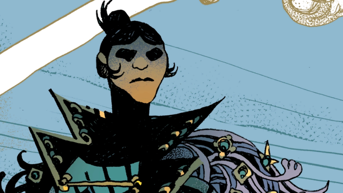
In this paper we introduces a new realtime level-of-detail deep-water animation scheme, which uses many different proven water models. In addition we show how to utilities today’s latest graphic hardware for realistic rendering of oceans.

Introduction

• Oceangraphic statistics based surface wave model for ocean waves (FFT)
• Physical correct surface wave model, taking depth into account, for realistic shorelines etc. (Shallow water waves)
• Constraint physical correct wave model for object interaction (Surface waves)
• Full Navier-Stokes simulated bump-map for surface tensions and similar turbulent effects (Navier-Stokes Equations) Our realistic (realtime) rendering of water includes all of the following visual features:
• View dependent water colouring (Colour of water)
• Global reflection/refraction (Reflection/Refraction)
• Local reflection/refraction (Reflection, Refraction)
• Caustics (Caustics) and Godrays (Godrays)
• Foam and spray (Foam, Spray and Bubbles)

Animation

The main philosophy behind our animation is that there is “no single model fitting all needs”. We haven’t tried to make one super model, but instead investigated how to blend between different types and levels of animation. We will first present all the difference models used, and then summaries of how and what we used them for.

FFT
First, we will describe the algorithm we’re using as a core of our sea animation. The algorithm is explained in detail in [2]. This model isn’t based on any physics models, but instead uses statistical models based on observations of the real sea. The method has been used commercially several times, for example for sea animation in the movies Titanic and Waterworld.

In this statistical model of sea, wave height is a random variable of horizontal position and time, h(X,t). It decomposes the wave heightfield into a set of sinus waves with different amplitudes and phases. While the model itself provides us with a tool to generate these amplitudes and phases, we use inverse Fast Fourier Transformation (FFT) as a mean to quickly evaluate the sum.

FFT is a fast version of discrete Fourier transformation, i.e. Fourier transformation that samples the input at regularly placed points. Description of both regular FT and FFT together with it’s interesting properties and working algorithms can be found in [6], which is also available online.

FFT allows us to quickly evaluate the following sum:

Here X is a horizontal position of a point whose height we are evaluating. The wave vector K is a vector pointing in the direction of travel of the given wave, with a magnitude k dependent on the length of the wave (l):

  k =2p /l

And the value of h (K,t) is a complex number representing both amplitude and phase of wave K at time t. Because we are using discrete Fourier transformation, there are only a finite number of waves and positions that enters our equations. If s is dimension of the heightfield we animate, and r is the resolution of the grid, then we can write:

  K = (k_x,k_z) = (2pn / s,2pm /s)

where n and m are integers in bounds –r/2 £ n,m < r/2. Note that for FFT, r must be power of two. For rendering the heightfield we need to calculate the gradient of the field to obtain normals. The traditional approach of computing finite difference between nearly placed grid points may be used, but it can be a poor approximation of the slope of waves with small wavelengths. Therefore, if we can afford it (in terms of computational power) it is better to use another FFT, this time evaluating the following sum:

Now that we know how to convert field of complex numbers representing wave amplitudes and phases into a heightfield, we need a way to create the amplitudes and phases themselves. Tessendorf [2] suggests using the Phillips spectrum for wind-driven waves. It is defined by the following equation:

In this equation, l = v² /g the largest possible wave arising from a continuous wind with speed v, g is the gravitational constant, Wˆ is direction of the wind and Kˆ is direction of the wave (i.e. normalized K). a is a numeric constant globally affecting heights of the waves. The last term in the equation (|Kˆ Wˆ|²) eliminates waves moving perpendicular to the wind direction. In this form, the resulting animation contains waves that adhere the wind direction, but move both with and against it, resulting in a lot of meeting waves (and opportunities for splashes and foam creation). If you prefer waves moving in one direction, you can modify this term to eliminate waves that moves opposite to the wind (i.e. the dot product is negative).

Also, to improve convergence properties of the spectrum, we can try to eliminate waves with very small length (w<<l) by multiplying the equation by the following term:

There are now two steps we have to do in order to prepare data for FFT – create the amplitudes and phases at time zero, and then animate the field. The first part can be accomplished using the equation:

Where z _r and z_i are two independent draws from a Gaussian random number generator with mean 0 and standard deviation 1.

Now, given time t, we can create a field of the frequency amplitudes (independently on previous time, which can be valuable):

Where w is angular frequency of wave k representing the speed at which the wave travels across the surface. You may wonder, what is the source of the right term in this equation? It’s there, because our resulting heights (result of the inverse FFT) are only real numbers (i.e. their imaginary part is equal to zero). It can be shown that for such a function, the following must holds for the amplitudes:

where * is the complex conjugate operator ¹.

As you may notice, there is one last piece missing in the jigsaw, and that’s value of w for a given wave. Since we are animating deep-water sea, there is a simple relation between w and the corresponding wave-vector K:

  w^{2 (K) =} gk

Here g is again the gravitational constant and k is the magnitude of vector K.

There are several modifications to this equation, perhaps the most useful for our purpose is taking depth d into account:

Also, if you intend to precalculate the animation, you might try to express each frequency as a multiply of the same basic angular frequency w₀ to ensure that the animation loops after a certain time. The results of implementing this set of equations, given above, are a tile of highly realistic sea surface. Given the properties of the FFT it can be seamlessly tiled over and over again. This is a very useful property, even though the tiling can be visible as a repeating pattern. We can improve this by choosing a larger grid, but this obviously comes at a computational expense. Tessendorf [3] mentions that for the Titanic animation, a grid size of 2048 was used. This is unfortunately too big to be animated in realtime on consumer-class computers. In our experiments we have been using mostly grid size 64, which inverse FFT can be computed quite fast. The size 128 however gives a (subjectively) much better visual result and will probably be the right size in case one are targeting today’s high-end configurations (and the water animation comprise significant part of the whole view).