Sponsored By
News
Splash screen for Marvel: Contest of Champions.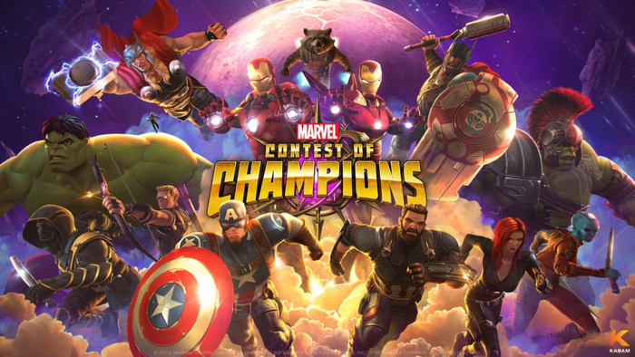
BusinessKabam is taking Marvel: Contest of Champions to 'alternative' app storesKabam is taking Marvel: Contest of Champions to 'alternative' app stores
Ahead of its 10th birthday, Marvel's mobile fighting game is leaving the iOS/Android playground to hang out in other app stores.


Latest News
Trending

Featured Blogs


Daily news, dev blogs, and stories from Game Developer straight to your inbox