Sponsored By
News
Key art for Capcom's Dragon's Dogma II.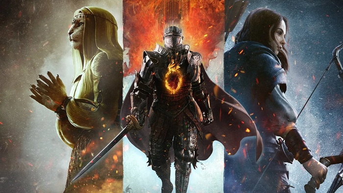
BusinessCapcom raises revenue goals in wake of Dragon's Dogma II's smash successCapcom raises revenue goals in wake of Dragon's Dogma II's smash success
With commercial hit after hit releasing in the last year, Capcom can't help but feel itself.


 Cécile Russeil.")


Latest News
Trending

Featured Blogs


Daily news, dev blogs, and stories from Game Developer straight to your inbox