Sponsored By
News
Key art for 2023's Cantata.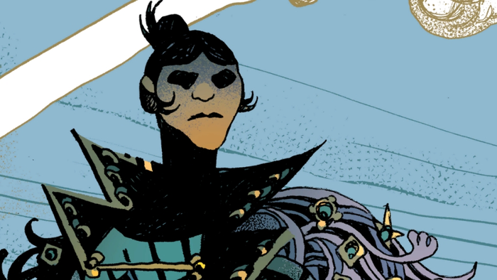
BusinessModern Wolf lays off six staff in studio restructuringModern Wolf lays off six staff in studio restructuring
The publisher's cuts come nearly a year after the launch of Cantata in mid-2023, and it's yet to release a game in 2024.


Latest News
Trending

Featured Blogs
Daily news, dev blogs, and stories from Game Developer straight to your inbox