Sponsored By
Latest News
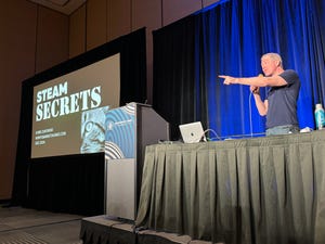
Raph Koster with a word bubble saying "Play the game I think is most fun: the game of makin ggames."
DesignRaph Koster wants developers to get back to 'the game of making games'
Raph Koster wants developers to get back to 'the game of making games'
Veteran game designer Raph Koster thinks there's a lot of room to explore what 'fun' is in game design.

Tips, Talks, and Highlights from GDC 2024
More from GDC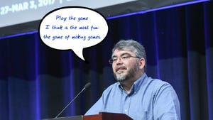


Get daily news, dev blogs, and stories from Game Developer straight to your inbox
Subscribe to Game Developer Newsletters to stay caught up with the latest news, design insights, marketing tips, and more


Game Developer Essentials
More resources for devs
Read Dev Blogs on Game Developer
See all

From Our Sponsors
LEARN MORE


Sponsored Content
Mar 8, 2024
.png?width=300&auto=webp&quality=80&disable=upscale)