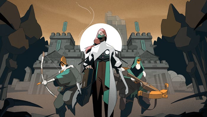
The rapid growth of CPU power opens possibilities for development of 3D games that feature realistic environment. The increase in the performance of graphics accelerators frees additional CPU cycles that can be used for real-time physical world modeling.

Game realism can be improved by simulating deformable objects or deformable surfaces. The list of common deformable objects and surfaces include:

• water (waves, streams, waterfalls), wind and splashes simulation;
• cloth (capes, flags, curtains), wind and wrinkle simulation;
• soil (mud, clay), imprint and crater simulation;
• vegetation (grass, trees), wind simulation.

Simulation of deformable objects results in unique experience of realistic never-the-same environment. Wind that causes waves and makes grass bend; objects that produce ripples when dropped in water; soil covered with footprints and explosion craters.

The user receives much richer sense of reality when the geometry of an object is modified rather than when anew or animated texture is mapped on to it because correctly deformed objects will look right from any angle and in any lighting conditions. Also deformed objects can block or reveal other objects behind them.

The implementation of deformable surfaces discussed in this article is intended for real-time 3D games that simulate realistic environment. The algorithm is optimized for AMD 3DNow! technology. Different implementations and their performance are discussed.

Physics of 2D surface deformation

Consider a grid that represents a simple 2D surface as shown on figure 1. Each vertex on the surface is connected with 6 neighbors to the north, east, southeast, south, west and northwest. This interconnection defines local topology. The neighboring vertices interact with each other by means of elastic forces (i.e. interconnections between vertices, depicted as solid lines on the figures, act as coil springs). In the initial (relaxed) state vertices are evenly spaced, and vectors S_RelaxE, S_RelaxSE, S_RelaxS specify distances between neighbors. In the relaxed state elastic forces between vertices are equal to zero.

Figure 1. 2D deformable surface at time t0=Dt, t1=2Dt and t2=3Dt.

When an external force (F_ext) is applied to a vertex on the surface at time t₀=Dt, the vertex starts moving and displaces to a new location time t₁=2Dt. This displacement produces elastic forces between local topological neighbors. The resulted elastic forces counter the displaced vertex motion and try to return the vertex to its original location. However according to the 3^rd Newton’s law the same forces but with opposite direction act upon neighboring vertices. So at time t₂=3Dt the neighbors get displaced, and entire cluster of vertices comes in motion. With time more and more vertices get involved in motion, representing wave propagation across the surface.

The 2D surface is characterized by the following parameters:

• local topology;
• global topology (i.e. plane, cylinder, sphere, etc.)
• vertex mass m;
• relaxation distances (S_RelaxE, S_RelaxSE, S_RelaxS);
• elasticity model (linear, exponential, etc.);
• elasticity constant (elasticity tensor E for anisotropic surfaces) E, E >= 0;
• damping constant (damping tensor D for anisotropic surfaces) d, 0 <= d <= 1.

Greater elasticity corresponds to faster deformation and stiffer body, while low elasticity corresponds to softer bodies.

Smaller damping represents faster relaxation or faster solidification for ductile surfaces.

This paper deals with plane isotropic surfaces combined from identical particles with mass m with six-neighbor local topology and linear elasticity model.

Figure 2. Vertex forces.

State of a vertex on the surface is characterized by coordinate vector S, velocity V, total internal (elastic) force F_Total and external force F_Ext.

The surface deformation is calculated for each vertex in the following way. First vertex displacement relative to the east, south and southeast neighbors is calculated:

DS_E = S_E - S - S_RelaxE

DS_S = S_S - S - S_RelaxS

DS_SE = S_SE - S - S_RelaxSE

Then elastic forces between local neighbors are evaluated:

F_E = Elasticity · DS_E

F_S = Elasticity · DS_S

F_SE = Elasticity · DS_SE

Total force acting on the vertex under consideration is:

F_Total = F_E + F_S + F_SE

According to the 3^rd Newton’s Law the vertex under consideration contributes to the total force acting on its neighbors:

F_TotalE = F_TotalE - F_E

F_TotalS = F_TotalS - F_S

F_TotalSE = F_TotalSE - F_SE

Notice that north, west and northwest elastic forces are not calculated directly. The total force for the vertex F_Total is updated automatically when north, west and northwest vertices are processed (3^rd Newton’s law).

Finally, when all vertices on the surface are processed (i.e. all internal forces evaluated) new coordinates are calculated for each vertex.

Acceleration is calculated from the 2^nd Newton’s law:

a = (F_Total + F_ext)/m

The rest is discrete numerical integration:

DV = a · Dt

V = V + DV

DS = V · Dt

S = S + DS

Lastly vertice velocity is adjusted in order to account for damping:

V = V · d